Tutorials
This tutorial will walk you through the basic workflow of Optinist. You can read through this tutorial and try running Optinst on our sample dataset. Then you will be ready to start using Optinist on your own data.
Loading Sample Data
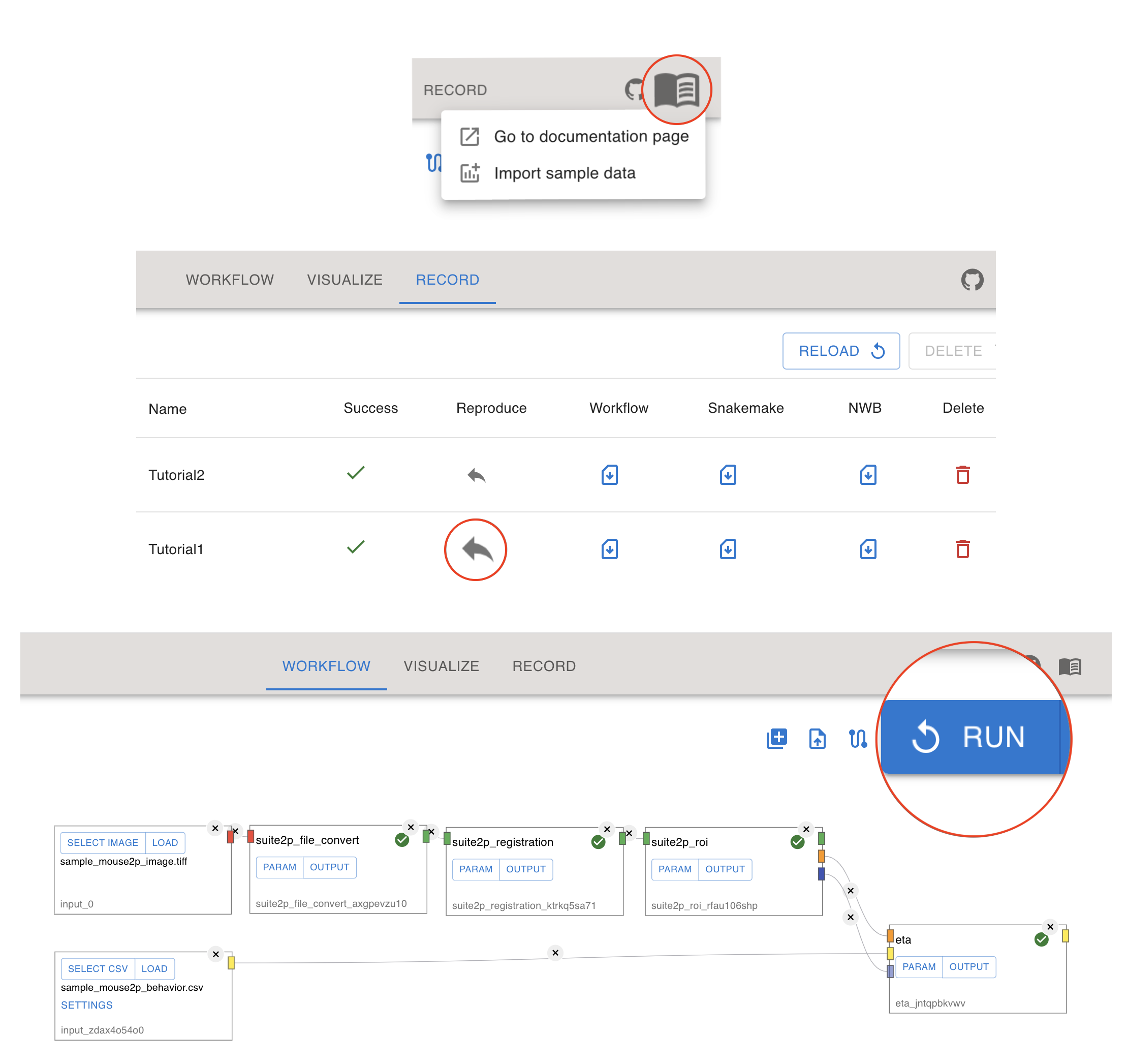
Let’s begin by loading some sample data. The Import sample data button can be found by first selecting the Documentation button. This action moves the sample data into your Optinist working directory.
Next, switch to the Record tab. This is where the records of all your workflows will be kept. You can conveniently reload any previous workflow from here. To load the tutorial workflow, select the Reproduce icon. Note that you can download the Workflow, Snakemake, and NWB files for use later.
Finally, switch back to the Workflow tab to see the loaded workflow. We’ll use Suite2P to register (motion correct) the imaging data and visualize the Event Triggered Average (ETA).
Since this will be the first time running this data on your computer, you’ll need to RUN the analysis.
Adding Nodes to your Workflow
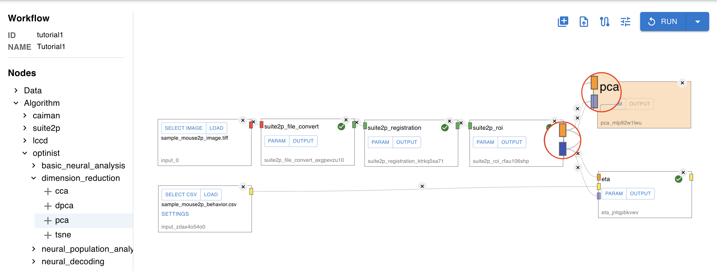
You can easily add new Data and Algorithm nodes from the left-hand side menu. Let’s practice by adding another type of analysis. Try selecting PCA (Principal Components Analysis) from the Algorithm menu. You’ll need to connect the nodes with the matching data type. Note that the opaque connector blocks are necessary, and the transparent blocks are optional. By connecting the blue blocks, only the ROIs that are confirmed as cells will be used for PCA.
Notice how the new node changes color. This will also happen anytime you change a parameter. You’ll need to Run the analysis again. Conveniently, Optinist checks which nodes are affected by changes and only runs what is necessary.
Checking the Data
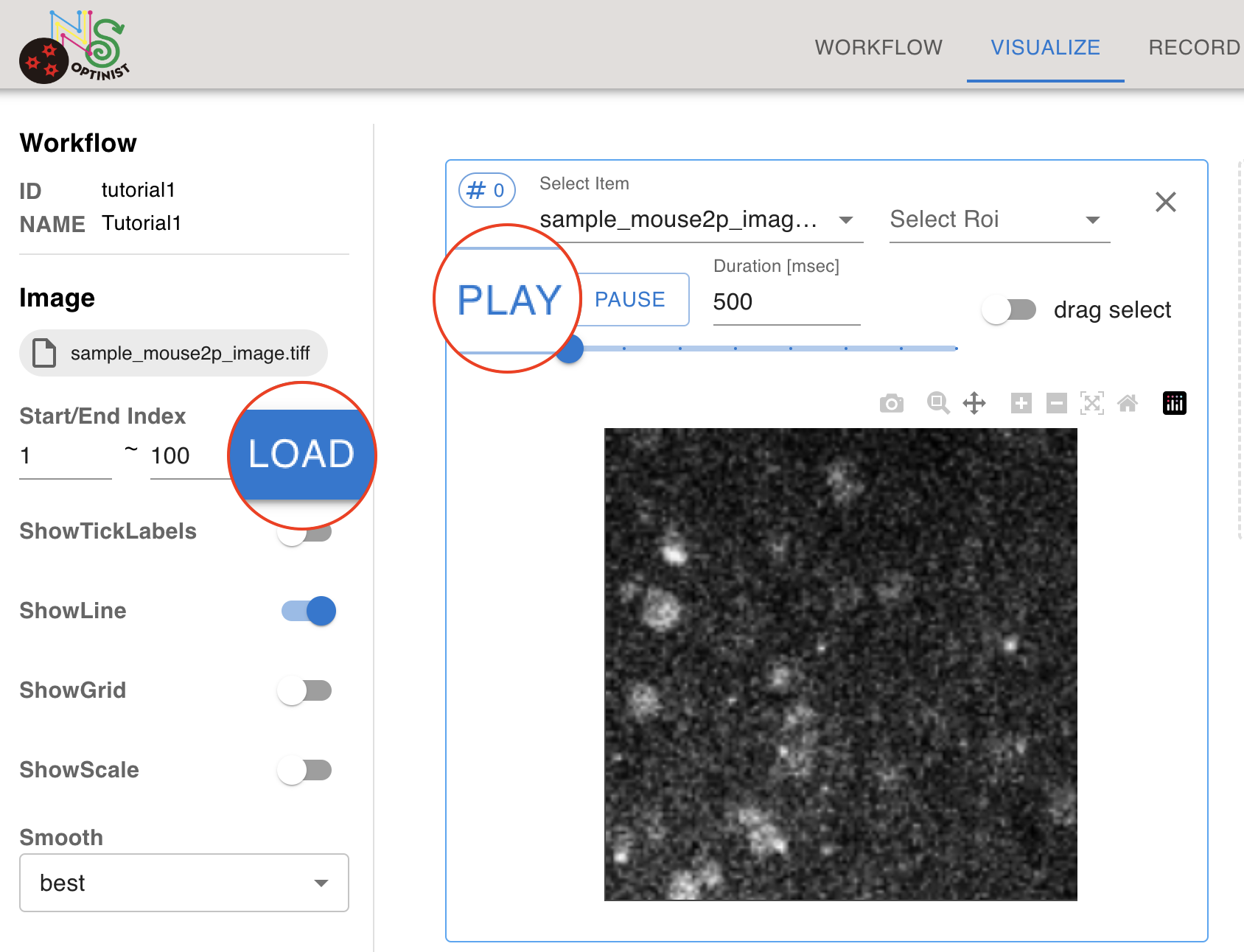
You may want to check the data after uploading it. Switch to the Visualize tab. Press the + icon to add a new box. Select the imaging data you want to see. If you adjust the start and end time, remember to press LOAD afterwards. You can also see the effectiveness of the motion correction by loading your original data and the motion corrected mc_images in side-by-side boxes.
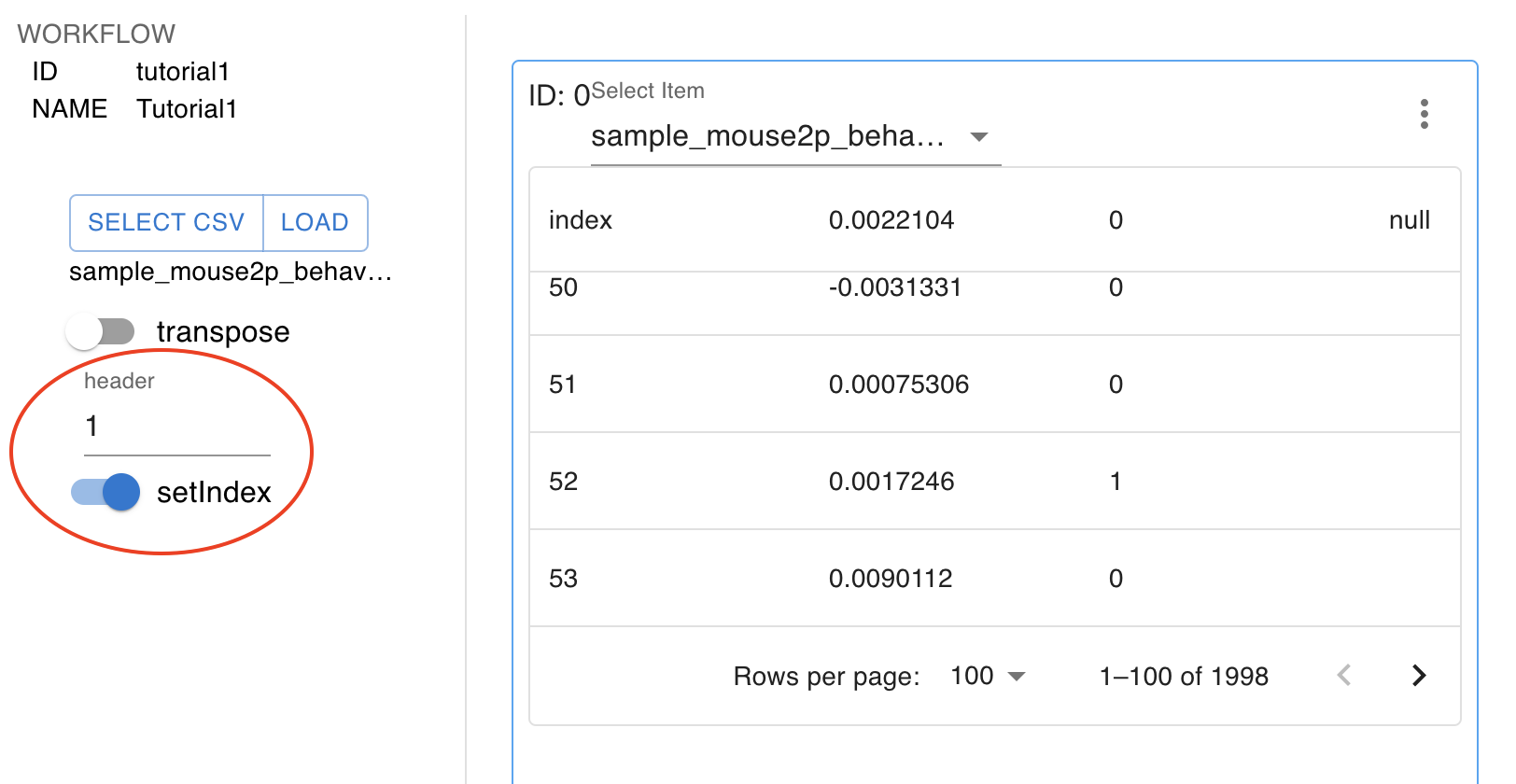
It is also possible to check your behavioural csv data in the Visualize tab. You can set the number of header rows to ignore at the top of your csv, and see how this affected the data indices.
Selecting ROIs
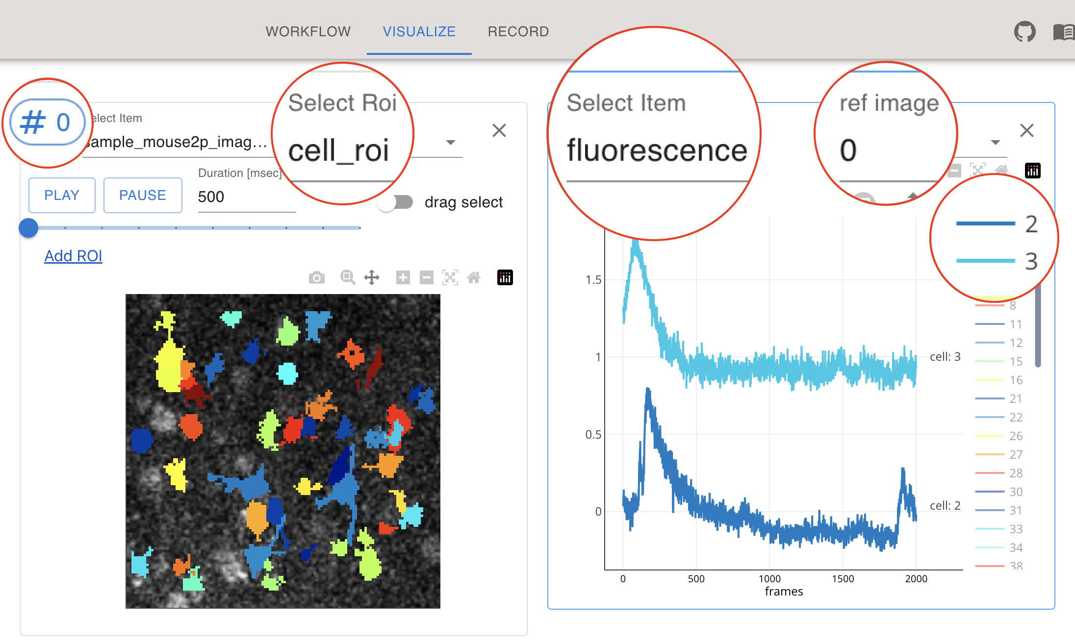
To visualise ROIs you first need to follow these steps:
Open a box and select your imaging dataset.
In the dropdown menu that appears to the right select the ROI type. Let’s start by checking
cell_roi.Open a second box and in the drop-down menu select
fluorescenceunder the suite2p_roi header.Link the two boxes using
Link to box (#), inputing the # of the other box.Select an ROI to see by clicking on the ROI mask or the ROI ID in the legend.
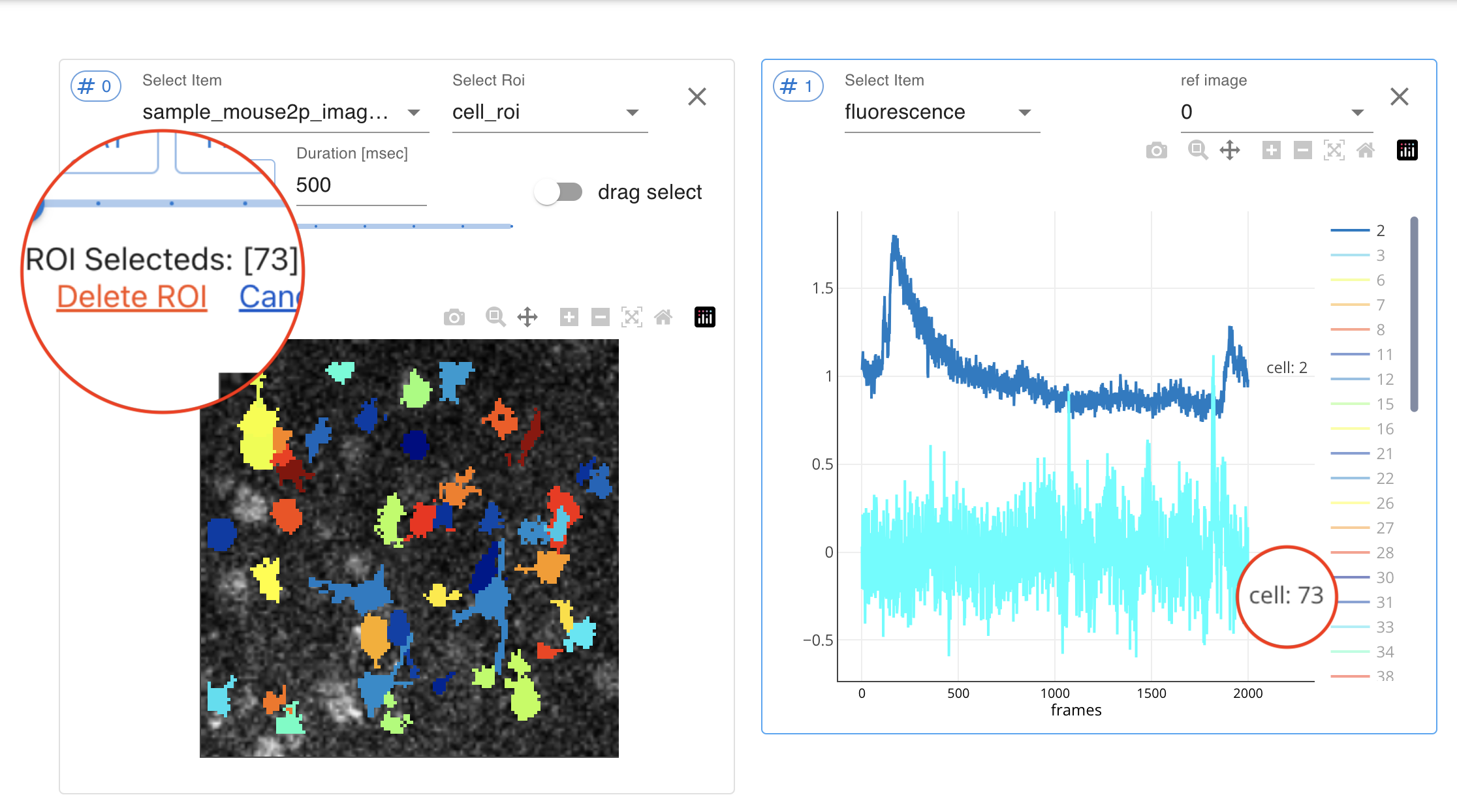
Optinist reproduces many of the amazing ROI editing functions of Suite2p.
You can move ROIs between the non_cell_roi and cell_roi categories using Add ROI and Delete ROI.
By clicking on more than one ROI mask, you can also Merge ROI. The selected ROIs will become a single new ROI with a new fluorescence time course will appear at the end of legend.
Visualising Analysis Algorithms
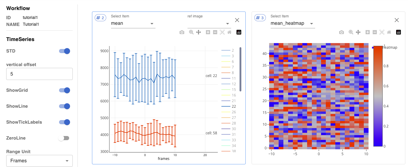
Finally, let’s check the ETA analysis. Open up a new box and select mean under the ETA header of the drop-down menu. Link this box to your data to only see the cell_roi data. Then select and ROI from the legend.
You’ll see the mean trace across all of the time points specified by 1s in the sample_mouse2p_behavior.csv file. Also std can be displayed by setting STD in the left side-bar to True.
You can also see a heatmap of all of the data using mean_heatmap. If you want to see longer pre- or post-stimulus periods, you can go back to Workflow, adjust the parameters and RUN again.
Practice with Tutorial 2 & 3
Now it’s your turn. Try loading Tutorial 2 from the Record tab. Tutorial 2 uses CaImAn, while Tutorial 3 uses LCCD. Give all the tutorials a try and compare different ROI produced on the same data. The results are surprisingly different! Don’t forget to RUN it the first time.
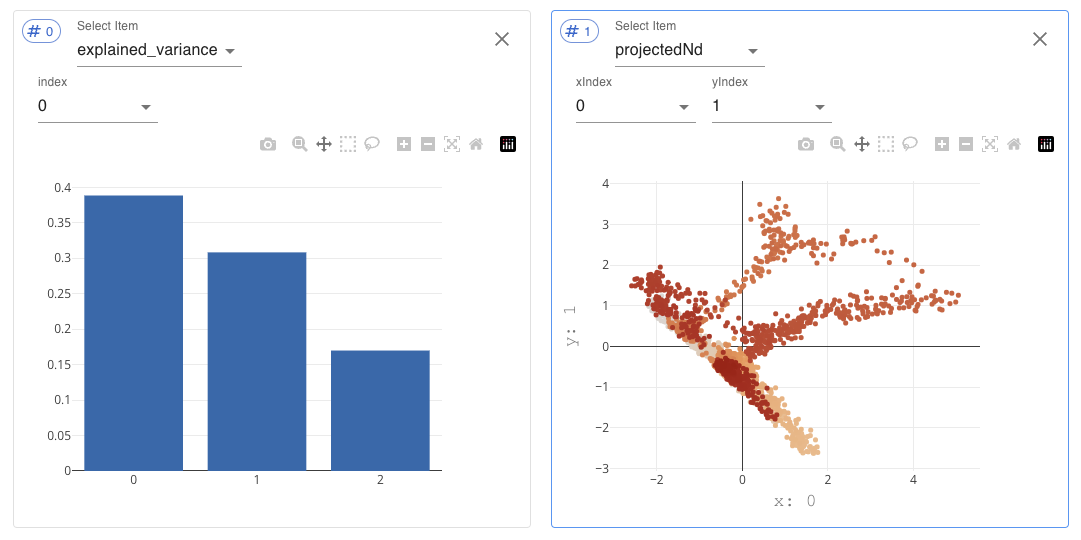
For Tutorial 2, if you check the Visualise output of explained_variance and projectedNd, you would recreate the figure below.